
Join faster with Couchbase Index Joins

[This article is reposted from my DZone article: https://dzone.com/articles/join-faster-with-couchbase-index-joins]

Good features in query language help you to optimize the data model, save space, and increase performance.
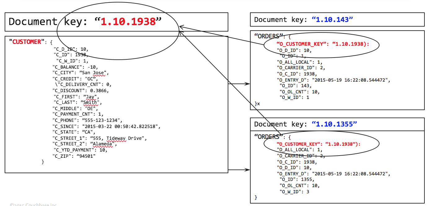
Normally, you’d have child table pointing to parent. For example, orders have the document key of the customer. So, starting with orders, you join customers to have the fully joined document which can be processed further.  
Image title

To get the list of orders by zipcode, you write the following query.
SELECT c.C_ZIP, COUNT(o.O_ID)
FROM ORDERS AS o LEFT OUTER JOIN CUSTOMER AS c
         ON KEYS o.O_CUSTOMER_KEY
GROUP BY c.C_ZIP
ORDER BY COUNT(1) desc;
This works like a charm. Let's look at the query plan.
We use the primary index on ORDERS to do the full scan.   For each document there, try to find the matching CUSTOMER document by using the ORDERS.O_CUSTOMER_KEY as the document key.  After the JOIN, grouping, aggregation and sorting follows.
[
  {
    "plan": {
      "#operator": "Sequence",
      "~children": [
        {
          "#operator": "Sequence",
          "~children": [
            {
              "#operator": "PrimaryScan",
              "index": "#primary",
              "keyspace": "ORDERS",
              "namespace": "default",
              "using": "gsi"
            },
            {
              "#operator": "Parallel",
              "~child": {
                "#operator": "Sequence",
                "~children": [
                  {
                    "#operator": "Fetch",
                    "as": "o",
                    "keyspace": "ORDERS",
                    "namespace": "default"
                  },
                  {
                    "#operator": "Join",
                    "as": "c",
                    "keyspace": "CUSTOMER",
                    "namespace": "default",
                    "on_keys": "(`o`.`O_CUSTOMER_KEY`)",
                    "outer": true
                  },
                  {
                    "#operator": "InitialGroup",
                    "aggregates": [
                      "count((`o`.`O_ID`))",
                      "count(1)"
                    ],
                    "group_keys": [
                      "(`c`.`C_ZIP`)"
                    ]
                  }
                ]
              }
            },
            {
              "#operator": "IntermediateGroup",
              "aggregates": [
                "count((`o`.`O_ID`))",
                "count(1)"
              ],
              "group_keys": [
                "(`c`.`C_ZIP`)"
              ]
            },
            {
              "#operator": "FinalGroup",
              "aggregates": [
                "count((`o`.`O_ID`))",
                "count(1)"
              ],
              "group_keys": [
                "(`c`.`C_ZIP`)"
              ]
            },
            {
              "#operator": "Parallel",
              "~child": {
                "#operator": "Sequence",
                "~children": [
                  {
                    "#operator": "InitialProject",
                    "result_terms": [
                      {
                        "expr": "(`c`.`C_ZIP`)"
                      },
                      {
                        "expr": "count((`o`.`O_ID`))"
                      }
                    ]
                  }
                ]
              }
            }
          ]
        },
        {
          "#operator": "Order",
          "sort_terms": [
            {
              "desc": true,
              "expr": "count(1)"
            }
          ]
        },
        {
          "#operator": "FinalProject"
        }
      ]
    },
    "text": "SELECT c.C_ZIP, COUNT(o.O_ID)\nFROM ORDERS AS o LEFT OUTER JOIN CUSTOMER AS c\n         ON KEYS o.O_CUSTOMER_KEY\nGROUP BY c.C_ZIP\nORDER BY COUNT(1) desc;"
  }
]
But, what if you’re interested California (CA) residents only? Simply add a predicate on the C_STATE field.
SELECT c.C_ZIP, COUNT(o.O_ID)
FROM ORDERS AS o LEFT OUTER JOIN CUSTOMER AS c
         ON KEYS o.O_CUSTOMER_KEY
WHERE c.C_STATE = "CA"
GROUP BY c.C_ZIP
ORDER BY COUNT(1) desc;
This works, except, we end up scanning all of the orders, whether the orders belong to California or not.  Only after the JOIN operation, we apply the C_STATE = "CA" filter.  In a large data set, this has negative performance impact.  What if we could improve the performance by limiting the amount of data accessed on ORDERS bucket.
This is exactly what the index-joins feature will help you do.  The alternate query is below.
SELECT c.C_ZIP, COUNT(o.O_ID)
FROM CUSTOMER AS c LEFT OUTER JOIN ORDERS AS o
         ON KEY o.O_CUSTOMER_KEY FOR c
WHERE c.C_STATE = "CA"
GROUP BY c.C_ZIP
ORDER BY COUNT(1) desc;
You do need an index on ORDERS.O_CUSTOMER_KEY.
To further improve the performance of this, you can create the index on CUSTOMER.C_STATE.
CREATE INDEX idx_okey ON ORDERS(O_CUSTOMER_KEY);
With these indexes, you get a plan like the following:
CREATE INDEX idx_cstate ON CUSTOMER(C_STATE);
Let's examine the explain. We use Two indexes idx_cstate which scans the CUSTOMER with the predicate (C_STATE = "CA") and then idx_okey which helps to find the matching document in ORDERS.
[
  {
    "plan": {
      "#operator": "Sequence",
      "~children": [
        {
          "#operator": "Sequence",
          "~children": [
            {
              "#operator": "IndexScan",
              "index": "idx_cstate",
              "index_id": "a3a663ec9928d888",
              "keyspace": "CUSTOMER",
              "namespace": "default",
              "spans": [
                {
                  "Range": {
                    "High": [
                      "\"CA\""
                    ],
                    "Inclusion": 3,
                    "Low": [
                      "\"CA\""
                    ]
                  }
                }
              ],
              "using": "gsi"
            },
            {
              "#operator": "Parallel",
              "~child": {
                "#operator": "Sequence",
                "~children": [
                  {
                    "#operator": "Fetch",
                    "as": "c",
                    "keyspace": "CUSTOMER",
                    "namespace": "default"
                  },
                  {
                    "#operator": "IndexJoin",
                    "as": "o",
                    "for": "c",
                    "keyspace": "ORDERS",
                    "namespace": "default",
                    "on_key": "(`o`.`O_CUSTOMER_KEY`)",
                    "outer": true,
                    "scan": {
                      "index": "idx_okey",
                      "index_id": "271ea96d9390e10d",
                      "using": "gsi"
                    }
                  },
                  {
                    "#operator": "Filter",
                    "condition": "((`c`.`C_STATE`) = \"CA\")"
                  },
                  {
                    "#operator": "InitialGroup",
                    "aggregates": [
                      "count((`o`.`O_ID`))",
                      "count(1)"
                    ],
                    "group_keys": [
                      "(`c`.`C_ZIP`)"
                    ]
                  }
                ]
              }
            },
            {
              "#operator": "IntermediateGroup",
              "aggregates": [
                "count((`o`.`O_ID`))",
                "count(1)"
              ],
              "group_keys": [
                "(`c`.`C_ZIP`)"
              ]
            },
            {
              "#operator": "FinalGroup",
              "aggregates": [
                "count((`o`.`O_ID`))",
                "count(1)"
              ],
              "group_keys": [
                "(`c`.`C_ZIP`)"
              ]
            },
            {
              "#operator": "Parallel",
              "~child": {
                "#operator": "Sequence",
                "~children": [
                  {
                    "#operator": "InitialProject",
                    "result_terms": [
                      {
                        "expr": "(`c`.`C_ZIP`)"
                      },
                      {
                        "expr": "count((`o`.`O_ID`))"
                      }
                    ]
                  }
                ]
              }
            }
          ]
        },
        {
          "#operator": "Order",
          "sort_terms": [
            {
              "desc": true,
              "expr": "count(1)"
            }
          ]
        },
        {
          "#operator": "FinalProject"
        }
      ]
    },
    "text": "SELECT c.C_ZIP, COUNT(o.O_ID)\nFROM CUSTOMER AS c LEFT OUTER JOIN ORDERS AS o\n         ON KEY o.O_CUSTOMER_KEY FOR c\nWHERE c.C_STATE = \"CA\"\nGROUP BY c.C_ZIP\nORDER BY COUNT(1) desc;"
  }
]
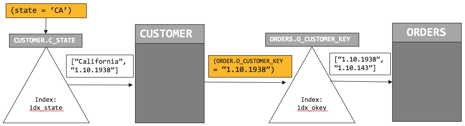
So, how does the this plan execute? Let’s look at the visual version of this.
Image title
We first initiate the index scan on CUSTOMER.idx_state and pushdown the filter (c.C_STATE = “CA”). Index scan returns list of qualified customers. In this case, the CUSTOMER document key is “1.10.1938”. We retrieve the CUSTOMER document and then initiate the index scan on ORDERS.idx_okey with the predicate on CUSTOMER document key (ORDERS.O_CUSTOMER_KEY = “1.10.1938”).  That scan returns the document key of the ORDERS, “1.10.143”.
Comparing plan 1 with plan 2, the plan to uses two indices to minimize amount of data to retrieve and process.  And therefore performs faster.
Index join feature is composable. You can use index join as part of any of join statements to help you navigate through your data model.   For example:
SELECT c.C_ZIP, COUNT(o.O_ID), COUNT(ol.OL_ORDER_ITEMS)
FROM CUSTOMER AS c LEFT OUTER JOIN ORDERS AS o
         ON KEY o.O_CUSTOMER_KEY FOR c
     INNER JOIN ORDER_LINE ol
      ON KEYS o.O_OL_ORDER_KEY
WHERE c.C_STATE = "CA"
GROUP BY c.C_ZIP
ORDER BY COUNT(1) desc;
Try it yourself easily.   I’ve given examples you can try out yourself on Couchbase 4.5 using the  beer-sample dataset shipped with it.  Checkout the slides at: http://bit.ly/2aCJOkd
Summary
Index joins help you to join tables from parent-to-child even when the parent document does not have a reference to its children documents. You can use this feature with INNER JOINS, LEFT OUTER JOINS. This feature is composable. You have a multi join statement, with only some of them exploiting index joins. 

Comments

Popular posts from this blog

Swami Vivekananda: The Monk That Nobody Sent to Chicago

  There’s a saying in Chicago: “We don’t want nobody that nobody sent.” This was the cold reception Swami Vivekananda faced when he arrived in the windy city in July 1893, determined to attend the World Parliament of Religions that September. He belonged to no organization, carried no letter of recommendation, his countrymen were nobody, and represented an alien religion to the Western world. As the days passed, his hope of attending the parliament dwindled. With money running out and the odds stacked against him, he left the Windy City and went to Boston, praying for a glimmer of opportunity.  Swamiji came to America to share India’s most profound gift: the wisdom of the Hindu sages, preserved through centuries of oral tradition and embodied by its monks. This was 1893, not 1993—India was under the British grip, its resources drained, and its spirit subdued. Swamiji’s mission was not just a cultural exchange; it was a bold step toward envisioning a future where India could re...

Why Should Databases Go Natural?

From search to CRM, applications are adopting natural language and intuitive interactions. Should databases follow? This article provides a strategic perspective. Amid the many technological evolutions in software and hardware (CISC/RISC, Internet, Cloud, and AI), one technology has endured:  Relational Database Systems   (RDBMS), aka SQL databases. For over 50 years, RDBMS has survived and thrived, overcoming many challenges. It has evolved and adopted beneficial features from emerging technologies like object-relational databases and now competes robustly with   NoSQL databases .  Today, RDBMS dominates the market, with four of the top five databases and seven of the top ten being relational. RDBMS has smartly borrowed ideas, like JSON support, from NoSQL, while NoSQL has also borrowed from RDBMS. NoSQL no longer rejects SQL. From a user perspective, all modern databases have SQL-inspired query language and a set of APIs. All applications manage the respective data...

iQ Interactive: Cool Things for Developers on Couchbase Capella iQ

  The landscape of software development is ever-evolving with the advent of new technologies. As we venture into 2023, natural language processing ( NLP ) is rapidly emerging as a pivotal aspect of programming. Unlike previous generations of tools that primarily aimed at enhancing coding productivity and code quality, the new generation of Artificial Intelligence ( GenAI ) tools, like iQ, is set to revolutionize every facet of a developer's workflow. This encompasses a wide range of activities: Reading, writing, and rewriting specifications Designing, prototyping, and coding Reviewing, refactoring, and verifying software Going through the iterative cycle of deploying, debugging, and improving the software Create a draft schema and sample data for any use case Natural language queries. Generate sample queries on a given dataset Fix the syntax error for a query Don't stop here. Let your imagination fly. Although the insights garnered from iQ are preliminary and should be treated ...